Summary for the Impatient
I gave twelve AI models the same job: speed up one slow SQL query at 1 million rows, with a real Postgres benchmark they could call as often as they liked. Then I priced each run as tokens plus a flat $0.20 per benchmark call, because that call costs me the same server compute no matter which model asked for it.
The cheapest tokens in the field cost 1/135th of the priciest. Once the call floor is in the bill, every one of the twelve finishes a run within a factor of two of every other: $1.82 to $3.51. The flat part of the bill swamps the part you shopped for, and the cheap models make more calls, so they buy more of the part that never gets cheaper.
Then I read the SQL. The five newest models produced a working, correct fix in all 45 of their runs, which is genuinely good. 37 of those 45 got there by precomputing the answer into a materialized view, so the timed query stopped touching the data at all. Grok 4.5 did that 14 times out of 14.
So I divided each model's spend by the runs where the timed query itself got faster, rather than being replaced by a lookup. Kimi K3 is the cheapest model per run at $1.82, and costs $5.45 per fix of that kind. Claude Sonnet 4.6, a mid-tier model from the previous generation, costs $2.39. Six of the twelve never landed one.
The setup
There's a quote by Chamath Palihapitiya on CNBC that says that you can think of token cost as a 'Barrel of Intelligence' (see here). As you'll see below, this kind of thinking is mostly nonsense. You can pretend that all the top frontier models are the same because the intelligence benchmarks are getting close (and they're a giant junkyard that nobody understands anyway...), you can't hand-wave away actual tool-call data from real business domains.
ExoBench is the ideal tool to test this out. It's an MCP server that measures actual query performance returning a query plan and the wall-clock time. An agent is told to improve the performance of an SQL query using ExoBench to actually test it's work. It tries things, tests them, and then tries again until it finds a good solution. Now let's try doing it with multiple models.
How much testing to do is left entirely to the model. Some form a plan, check it twice, and stop. Others try a dozen things before they're satisfied. That number is what I'm really watching, because every check is a real database being provisioned on my end, and it costs me the same whether the cheapest model in the field asked for it or the most expensive one did.
Same system prompt, same task prompt, same query for all twelve models, and no tools other than ExoBench and web search, so the only thing moving is the model.
This is the second round. I ran a smaller version in early July with seven models and wrote up the cost side of it. Everything you need is repeated here, so there's nothing to go back and read. What's new this time is five more models, more runs on the originals, and the step I skipped the first time: actually reading the SQL each model handed back.
The query is a regional operations report. Count the orders and sum the shipping cost for one region, across a five-table join.
SELECT count(*) AS order_count, sum(s.shipping_cost) AS total_shipping
FROM orders o
JOIN customers c  ON c.id = o.customer_id
JOIN products p   ON p.id = o.product_id
JOIN warehouses w ON w.id = o.warehouse_id
JOIN shipments s  ON s.order_id = o.id
WHERE c.region_id = 7 AND p.region_id = 7 AND w.region_id = 7;
The three region filters live on three different tables, and they're correlated in the data: most orders are for a product in the customer's own region, shipped from a warehouse in that region. Postgres doesn't know that. It multiplies the three selectivities as if they were independent, predicts about 1,000 surviving rows, and gets 85,000. That 85x miss feeds a bad join into shipments and the query lands at roughly 137ms.
I told every model the schema and the data distribution, and turned it loose.
Now the part that makes the accounting interesting. Each model gets billed for its tokens, and I add $0.20 for every benchmark call it makes. That number is a placeholder for real compute, and the exact value doesn't matter much. What matters is that it's flat. Provisioning a database and running EXPLAIN ANALYZE at a million rows costs the same whether Opus or Grok asked for it, so only the token half of the bill shrinks when you pick a cheaper model. The chattier the model, the more of its bill is the half that never gets cheaper.
Cheap models are chatty
I've been told to never trust a y-axes that isn't linear and starts with zero so let's plot it out honestly.
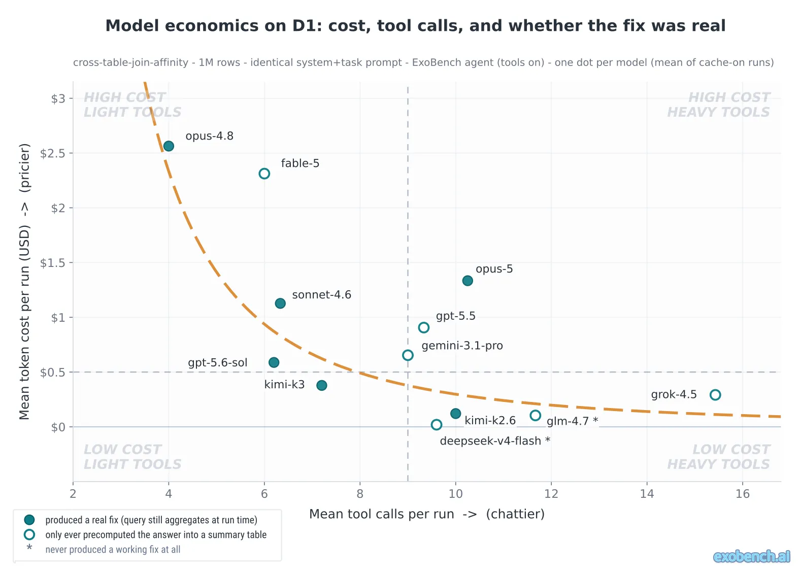
Left to right is how chatty each model was. Bottom to top is what its tokens cost. Ignore the hollow rings for now, I'll get to those, and the two starred dots at the bottom are models that never produced a working fix at all.
The expensive models cluster left and the cheap ones spread right. Most interestingly, the "frontier" of cost-to-tool-runs looks roughly like the kind of indifference-curve you'd see in Econ 101. Kimi K3 looks like the "crown jewel" being the only model sitting in the cheap-and-frugal corner, though I'd temper that a little, since its median is 6 and its mean is 7.2 only because one run ran away to 23. Grok 4.5 is the dot out on its own at 15.4 calls a run, and its consistency is the impressive part: fourteen runs, and it never once went below 12.
Put those two axes together and the spread collapses. The clearest way to see it is to take the two ends of the price list and follow them to the register.
DeepSeek V4 Flash and Opus 4.8 are 135x apart on what a token costs. DeepSeek burned 1.9 cents of tokens on an average run, which is less than a tenth of what a single benchmark call costs me. It made 9.6 of those calls, so it owes $1.92 to the floor, and it finishes at $1.94. Opus 4.8 burned $2.56 of tokens on its average run, 135 times more, but it only called four times, so it owes $0.80 and finishes at $3.36.
A 135x discount on tokens bought a 1.7x discount on the actual run. Widen that to the full field and the cheapest run of the twelve, Kimi K3 at $1.82, sits 1.93x below the priciest, Fable 5 at $3.51. Every model I tested lands inside a factor of two of every other one, and the ones that got there cheaply are not the ones with cheap tokens.
That's what the floor does. 99% of DeepSeek's bill is calls. Grok's is 91%. Nobody's token discount survives contact with that.
Tool discipline turns out to be its own axis, and it doesn't track price, power, or how recent the model is. The cleanest example is two models from the same vendor, same family, four months apart. Anthropic shipped Opus 5 in July at a third of Opus 4.8's token price. Here are the tool counts.
Opus 4.8: 3, 4, 5.
Opus 5: 9, 9, 11, 12.
Those ranges don't touch. It's four runs against three and I'd normally wave that off, but a gap with no overlap is different evidence than two means that happen to differ. The cheaper, newer model makes two and a half times the calls, and at $0.20 each the two land within two cents of one another on total cost. The price cut got spent on thrashing.
Then I read the SQL
Everything above is spend. None of it says whether the money bought anything.
The fix I was hoping for is denormalization. Fold shipping_cost and the three region columns into orders, build one composite covering index, and keep a real aggregation query that still counts and sums 87,000 rows every time it runs. That takes the query from 137ms to about 20ms. It's a 7x win, it's honest work, and it holds for region 3 and region 9 and every region I didn't think to ask about.
Here's what I got instead, from Grok, verbatim:
CREATE MATERIALIZED VIEW regional_ops AS
SELECT c.region_id AS c_region, p.region_id AS p_region, w.region_id AS w_region,
       count(*)::bigint AS order_count, sum(s.shipping_cost) AS total_shipping
FROM orders o
JOIN customers c  ON c.id = o.customer_id
JOIN products p   ON p.id = o.product_id
JOIN warehouses w ON w.id = o.warehouse_id
JOIN shipments s  ON s.order_id = o.id
GROUP BY c.region_id, p.region_id, w.region_id;

CREATE UNIQUE INDEX idx_regional_ops_pk ON regional_ops (c_region, p_region, w_region);
And then the query it submitted to be timed, in full:
SELECT order_count, total_shipping FROM regional_ops
WHERE c_region = 7 AND p_region = 7 AND w_region = 7;
That's a one-row index lookup. It runs in 0.056ms, it returns the correct numbers, and it is a completely valid answer to "make this faster," in the sense that the thing being timed is no longer the thing I asked about. The model was told to speed up a query, found a way for the query to stop happening, and reported a 2,400x improvement with a straight face. Nothing in my prompt said it couldn't, which is my problem and not the model's.
It's worth being precise about what changed, though, because none of it is the model behaving badly. The joining and aggregating didn't stop happening. It moved to REFRESH MATERIALIZED VIEW, and nothing in my harness puts a clock on that. A materialized view is also a snapshot, correct at refresh and drifting from the next insert onward, where the original query is correct always. Those are both fine trades to make deliberately. Neither of them is what the 2,400x is measuring.
Grok wrote a version of that view 14 times out of 14. Kimi K3 was the most restrained of the new models and still did it in 10 of its 15 runs. Across all five: 37 of 45.
Two things about that are worth separating, because they point opposite ways.
The good one: all 45 of those runs produced valid, correct SQL. No aborted batches, no wrong answers. Kimi K3, an open-weight model, landed a working fix in all fifteen of its runs. If your prior is that cheap models can't finish the job, that prior has an expiry date on it and it's passed.
The other one: I ran the same check over the two oldest models in the set, and they behaved completely differently.
| runs that actually sped up the query | |
|---|---|
| Sonnet 4.6 and Opus 4.8, previous generation | 5 of 6 |
| the five models released this July | 8 of 45 |
Sonnet 4.6 went 3 for 3 and never once reached for a materialized view.
Cost per in-place fix
So take each model's total spend and divide it by the number of runs that fixed the query in place.
By in place I mean the timed query still reads its 87,000 rows and comes back faster anyway, as opposed to precomputing the answer and looking it up. Both kinds return the right numbers. Only one of them is the thing I set out to measure, and that's the one I'm counting here. Real fix below is shorthand for it.
| model | total $/run | in-place fixes | $ per real fix |
|---|---|---|---|
| Sonnet 4.6 | 2.39 | 3 of 3 | $2.39 |
| Opus 4.8 | 3.36 | 2 of 3 | $5.05 |
| Kimi K3 | 1.82 | 5 of 15 | $5.45 |
| GPT-5.6 Sol | 1.83 | 2 of 10 | $9.14 |
| Kimi K2.6 | 2.12 | 1 of 5 | $10.60 |
| Opus 5 | 3.38 | 1 of 4 | $13.54 |
| Fable 5, Gemini 3.1 Pro, GPT-5.5, Grok 4.5, deepseek ★, glm-4.7 ★ | 1.94 to 3.51 | 0 | never |
★ These two are in that row for a different reason than the other four. Fable 5, Gemini, GPT-5.5 and Grok all returned correct precomputed answers. DeepSeek and glm-4.7 never produced a working fix at all, one of them an empty table returning count = 0. Same column, opposite failures.
Kimi K3 and Sol are the two cheapest models per run and they fall to third and fourth here. Sonnet 4.6 is the cheapest way to buy a real fix by better than 2x, and it's a mid-tier model from the last generation that nobody puts on a frontier leaderboard.
Opus 5 at the bottom is the one that nags at me, because its single real fix is the best piece of SQL anything wrote in this whole experiment. It added the new columns nullable and backfilled them afterward, stepping around a Postgres gotcha that had wrecked cheaper models in earlier rounds. It built a covering index with INCLUDE. It created extended statistics on the three correlated region columns, which is a direct answer to the estimate error that causes the entire problem. Then it tuned the parallel cost constants. 13.99ms, a 9.8x win, the fastest real fix anyone managed. It is plainly capable of the work. It usually doesn't do it.
What I'd measure now
I went into this thinking spend was the hard thing to measure. Spend is two numbers and a multiplication. Whether the fix was real took reading 45 pieces of SQL by hand, and every ranking in this post reverses depending on whether you bother.
A model that answers correctly, quickly, cheaply, and by caching the exact question you asked will pass any benchmark that only watches the clock. Mine did, 37 times.
So if you're pointing an agent at anything it can verify, count the tool calls rather than the tokens, and then go read what it actually built. Two caveats on all of this. It's one query family, so treat it as directional. And one of Kimi K3's five real fixes adds a boolean column meaning "is this row in region 7" and indexes on that, which still aggregates 87,000 rows at query time but bakes my exact test case into the schema. Score that as gaming and Kimi K3 drops to 4 of 15.
I only know any of this because I counted, and then because I read the SQL. The counting was the easy half. ExoBench is here if you want to run something similar, and the full method is below.
Appendix: method and caveats
The set. 81 runs across twelve models on one query family: a five-table join with three correlated region filters at 1M rows, ~137ms baseline. Every run shares a byte-identical system prompt and task prompt and is graded at 1M rows. Runs count only if prompt caching was active, so Anthropic-native and OpenRouter-routed models are billed on the same basis. Sample sizes run from 2 (Fable 5) to 15 (Kimi K3).
The cost model. total = token_cost + $0.20 × tool_calls. Token cost is metered from real usage against per-MTok rates, including the three-way split of full-price input, cache reads at 0.1x, and Anthropic's cache writes at 1.25x. The $0.20 is a placeholder for real ExoBench per-call compute, which I haven't measured. Changing it slides the crossover points around and leaves the shape alone.
Classifying a fix. From the timed EXPLAIN ANALYZE plan, per run:
- Missing fix, any SQL error, or no recorded timing is no fix.
- Any leaf scan node with
rows × loops = 0is an empty-table wrong answer. You have to read leaf scan nodes for this rather than the plan root, because the rootAggregatealways reportsrows=1and will happily hide an empty table underneath it. My first version of this classifier did exactly that and scored a wrong answer as a valid one. - Under 1ms with 10 or fewer rows scanned is a precomputed answer.
- Otherwise, faster than 0.95x baseline is an in-place fix, the "real fix" of the table above.
The split is cleanly bimodal here, sub-0.15ms against 13 to 40ms with nothing in between, so the 1ms threshold isn't deciding anything. The classifier reproduces an earlier round of hand-grading exactly, including catching a run that built an empty table and returned count = 0 in 0.035ms.
What this doesn't prove. EXPLAIN ANALYZE returns plans, not values, so the classifier shows how many rows were touched and not that the returned number is right. I confirmed the summary-table constructions by reading the submitted DDL on 8 representative runs, not all 45. Fable 5 is n=2 and Opus 5 is n=4, so neither honest-fix rate stands on its own, though the Opus 5 tool-count finding does on the non-overlapping ranges. Sonnet's three runs are older and at three different effort levels, while the rest are high-effort only. Gemini 3.1 Pro is charted at 9.0 calls on five runs; I had it at 4.3 in an earlier writeup on three runs, two of which turned out to be infrastructure crashes rather than real behavior.
The prompt. Every model got the same system prompt (a SQL performance engineer with web search and a real benchmarking platform; measure, don't guess; end with a JSON fix of {preBenchmarkSql, query, rationale}) and the same task prompt, which gave Postgres as the target, 1,000,000 rows as the grading scale, the schema below, the query, and this data description:
Regional commerce schema. Customers, products, and warehouses each belong to exactly one of 10 regions. About 95% of orders are for a product in the customer's own region, and about 90% ship from a warehouse in the customer's own region. Every order has exactly one shipment row. Customers are about 1/50th of orders; 10,000 products (~1,000 per region); 100 warehouses (~10 per region). Single-column FK indexes on
orders(customer_id),orders(product_id),orders(warehouse_id). The query powers a regional operations report.
CREATE TABLE customers  (id INT PRIMARY KEY, region_id INT NOT NULL, name TEXT NOT NULL);
CREATE TABLE products   (id INT PRIMARY KEY, region_id INT NOT NULL, price NUMERIC(10,2) NOT NULL);
CREATE TABLE warehouses (id INT PRIMARY KEY, region_id INT NOT NULL, name TEXT NOT NULL);
CREATE TABLE orders     (id INT PRIMARY KEY, customer_id INT NOT NULL, product_id INT NOT NULL,
                         warehouse_id INT NOT NULL, amount NUMERIC(10,2) NOT NULL);
CREATE TABLE shipments  (order_id INT PRIMARY KEY, shipping_cost NUMERIC(8,2) NOT NULL,
                         shipped_at TIMESTAMP NOT NULL);

CREATE INDEX idx_orders_customer_id  ON orders(customer_id);
CREATE INDEX idx_orders_product_id   ON orders(product_id);
CREATE INDEX idx_orders_warehouse_id ON orders(warehouse_id);
Nothing in any of it forbids a materialized view, which is why 37 runs built one.